How to Create Progress Bars in Excel for Task and Project Tracking

Tracking task or project completion in Excel becomes much easier when you use visual progress bars. Instead of scanning numbers, you can quickly see which tasks are on track, identify bottlenecks, and prioritize work. Excel offers multiple ways to create progress bars, including built-in conditional formatting, stacked bar charts, text-based formulas, and weighted checkboxes.

1. Create Progress Bars Using Conditional Formatting Data Bars

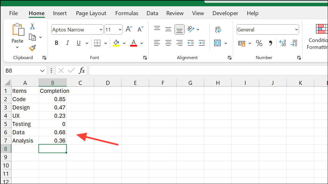
Step 1: Enter your tasks in one column (e.g., Column A) and their completion percentages in an adjacent column (e.g., Column B) as decimals (0.25 for 25%).

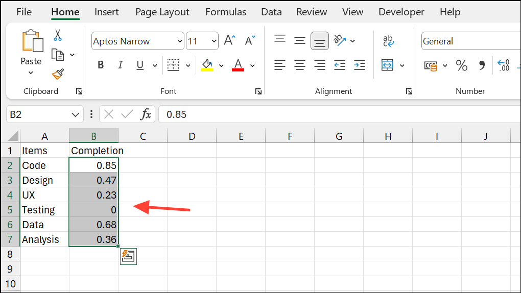
Step 2: Select the cells containing the percentages (e.g., B2:B11).

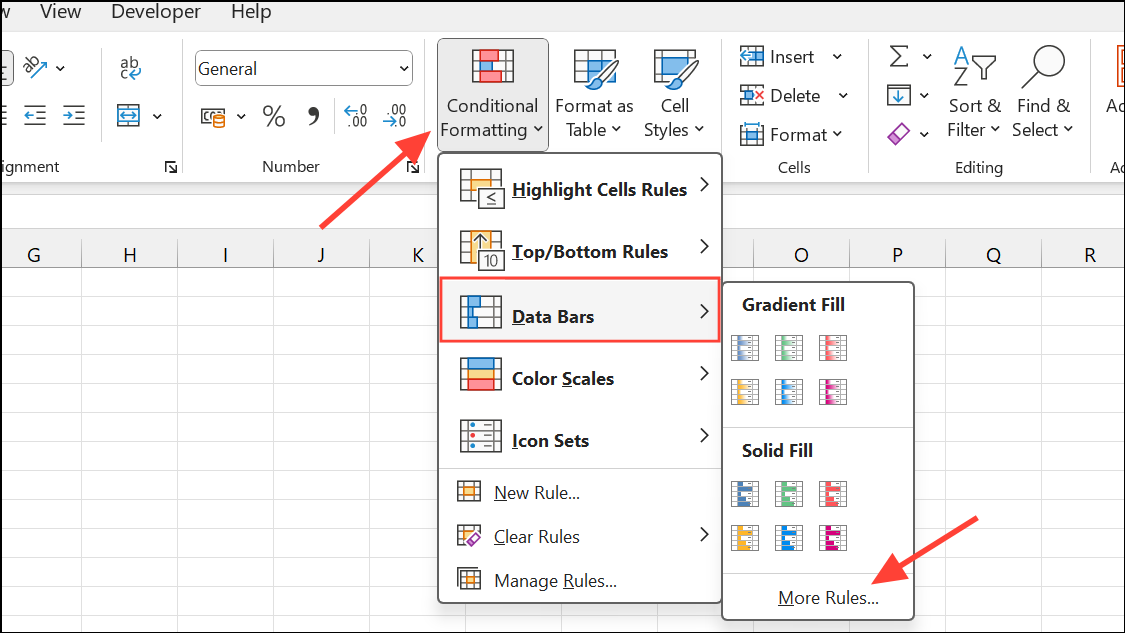
Step 3: Go to the Home tab, click Conditional Formatting > Data Bars > More Rules.

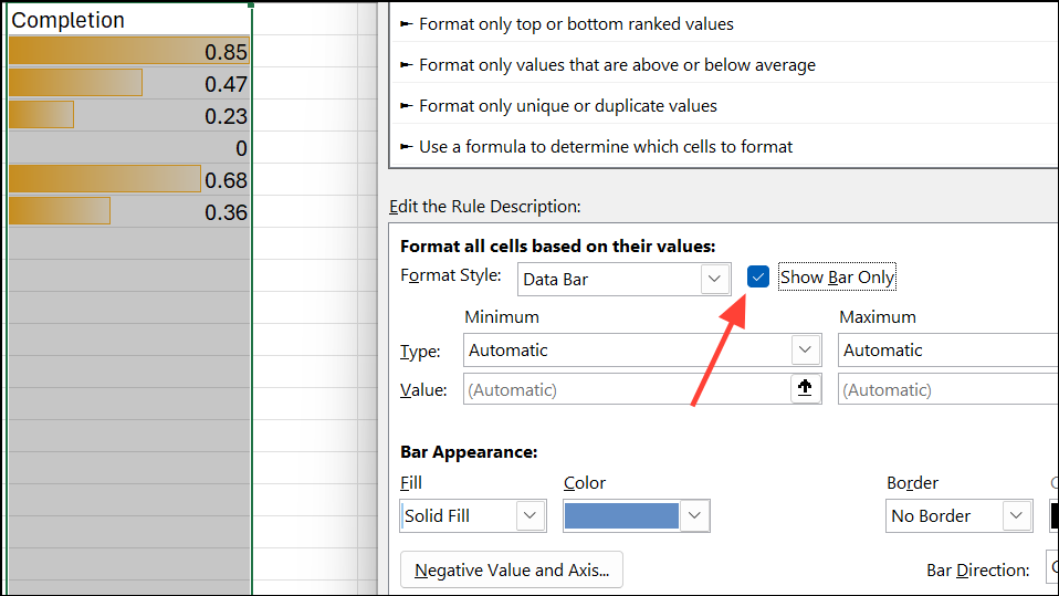
Step 4: Set Minimum and Maximum types to Number, enter 0 and 1 respectively, and pick a fill color.

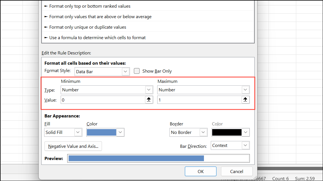
Step 5: Click OK. Each cell now displays a bar proportional to the completion percentage. Updating values automatically resizes the bars.

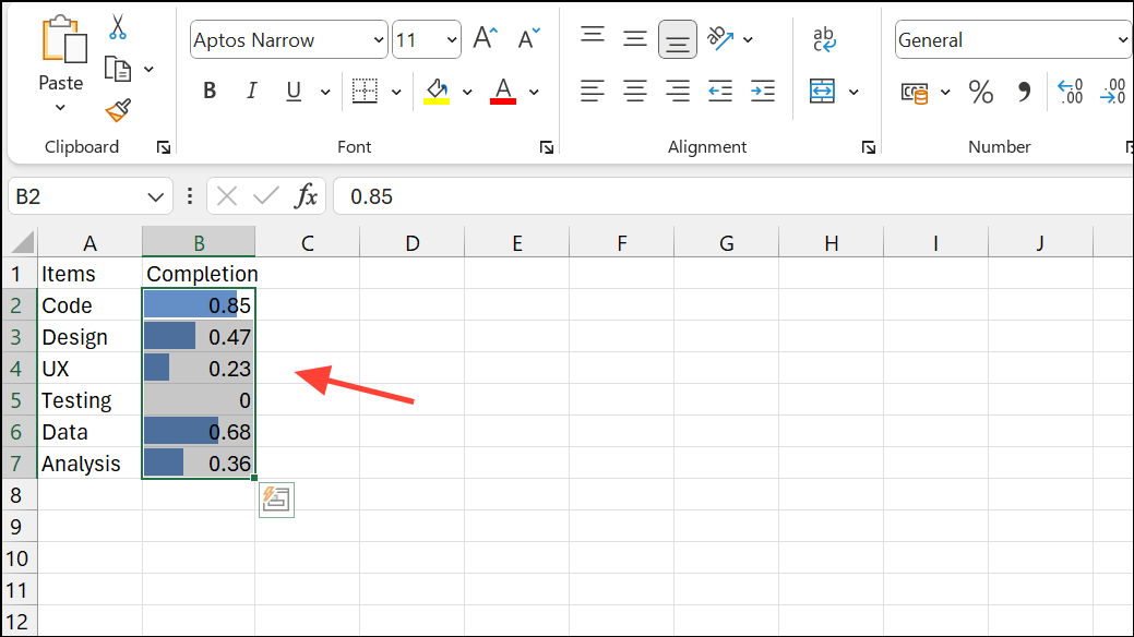
Step 6: Adjust column width or row height for readability. Optionally, check Show Bar Only to hide numeric values.

2. Customize Progress Bars for Thresholds

You can highlight tasks that exceed certain limits, such as over-completion.

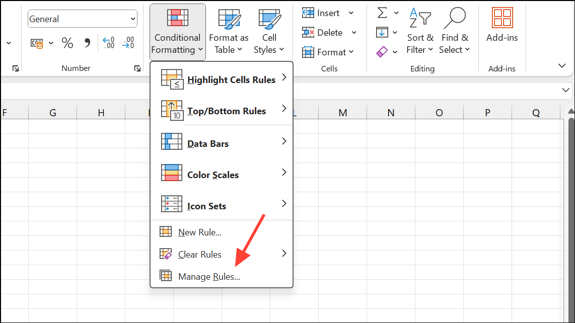
Step 1: Select your percentage cells and go to Conditional Formatting > Manage Rules > New Rule.

Step 2: Choose Use a formula to determine which cells to format.

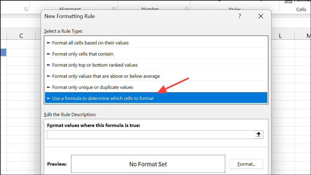
Step 3: Enter a formula like =B2>1 to target over-100% values.

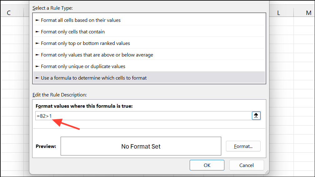
Step 4: Click Format, choose a red fill, and move this rule above the data bar rule to ensure it takes precedence.

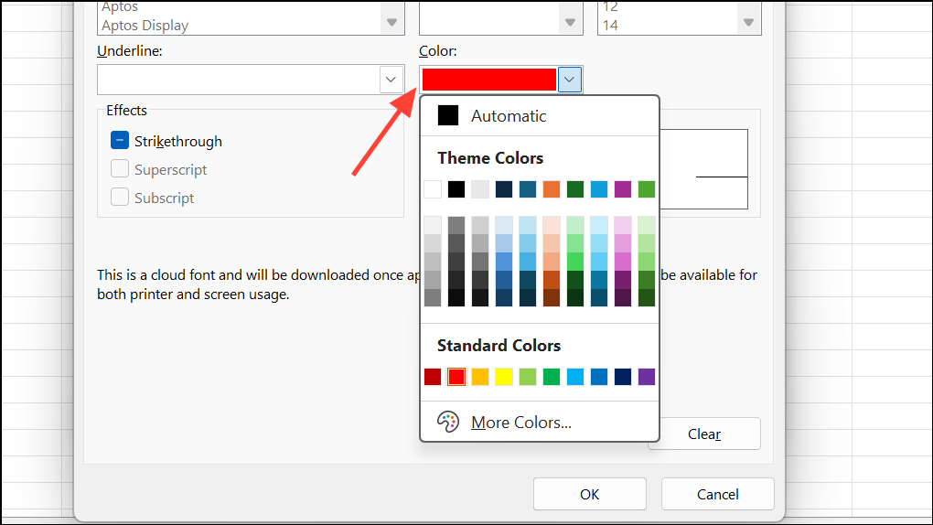
This draws immediate attention to tasks exceeding 100% completion.

3. Build Accurate Progress Bars with Stacked Bar Charts

For precise or more visually prominent bars:

Step 1: Organize data into three columns: task name, progress percentage, and remaining percentage (=1-B2).

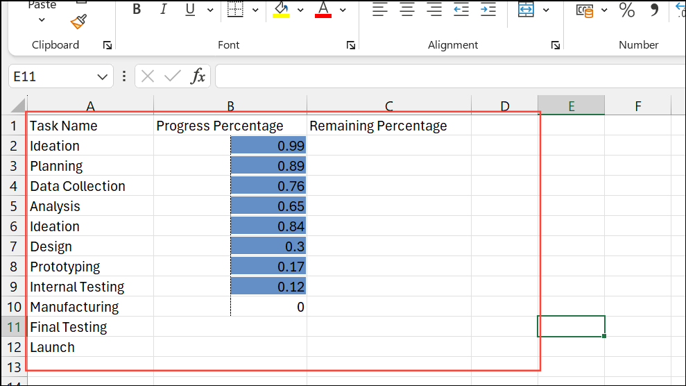
Step 2: Highlight the progress and remaining columns, go to Insert > Bar Chart > Stacked Bar.

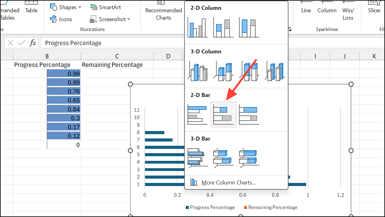
Step 3: Format the “Remaining” series with a light gray or no fill, and the “Progress” series with a solid color.

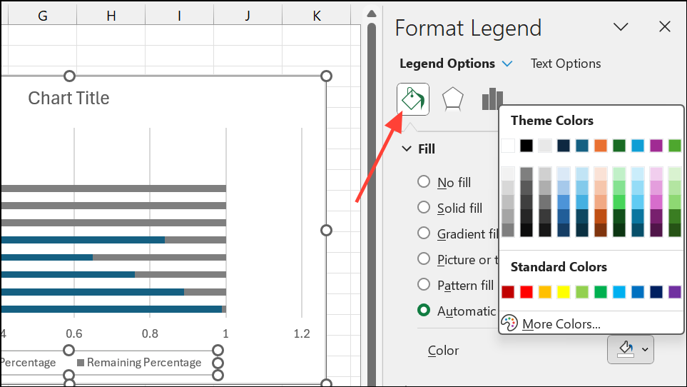
Step 4: Remove unnecessary legends or chart titles and add data labels if desired. The chart updates dynamically with your data.

4. Create Text-Based Progress Bars Using Formulas

For a compact, minimalist display:

Step 1: In a helper column, use:

=REPT("▓", B2*10) & REPT("-", (1-B2)*10)

Each “▓” represents 10% completion, and “-” represents remaining progress.

Step 2: Update the formula range to match your data. Bars update automatically when percentages change.

This is ideal for dashboards where space is limited.

5. Use Checkboxes and Weighted Completion

When tasks have different importance or durations:

Step 1: List tasks, assign weights (e.g., 60%, 20%, 10%, 10%), and add checkboxes for completion.

Step 2: Calculate total weighted completion using:

=SUMPRODUCT(--(status_range=TRUE), weight_range)

Or, with dynamic arrays:

=BYROW(status * {0.6,0.2,0.1,0.1}, LAMBDA(x, SUM(x)))

Visualize the result with any conditional formatting or chart-based method. This ensures each task contributes appropriately to overall progress.

Conclusion

Progress bars in Excel are powerful tools for quickly assessing task and project completion. Whether you use conditional formatting, stacked charts, text-based formulas, or weighted checkboxes, these visual indicators make your spreadsheets more actionable. Regularly updating your data ensures accurate, meaningful visualizations that help manage workloads efficiently.